
In June, I attended the Durham HPC Days event hosted at Durham University while representing the Met Office. I’ve heard the phrase “the world of HPC is surprisingly small” a few times, and it’s during these events you realise why. So, when you get reunite with those people from across the country who you’ve seen at a few of these things, it actually makes for a really fun week. More reconnecting than networking. Aside from that, this is my account of some technical highlights from my time in Durham.
Node-level Performance Optimisation
This session was run by Thomas Gruber, inventor of the LIKWID (Like I Knew What I’m Doing) profiling tool. The workshop was split into three sections. The first was focusing on computer architecture and memory hierarchy as well as parallelism technologies on the core. The second considered the basics of performance engineering, while working to the constraints of the architecture, and the tools used to assess that performance. The third and final session was a hands on session with the LIKWID profiling tool.
Session one revolved mostly around the basics of core and uncore architecture and features with an emphasis on their performance enhancing and limiting characteristics. In-core features were discussed first, with the implementation of pipelining and superscalar execution which achieve much greater throughput by employing out-of-order execution to compensate for the latency in instructions. This allows for concurrent execution and an improved steady state of multiple instructions per cycle. Also discussed was 2-way Simultaneous Multi-Threading (SMT), Fused Multiply-Add (FMA) and Single Instruction Multiple Data (SIMD). SIMD allows execution of a single instruction on many bits of data. The amount of data is dependent on the width of the register. For AVX, the register is 256 bits, and for AVX512, the register is 512 bits. These technologies add up to give a formula for the peak performance of a core $P_{core}$ for a particular precision, which is given as
$$ P_{core}=n_{super}^{FP} \cdot n_{FMA} \cdot n_{SIMD} \cdot f, $$
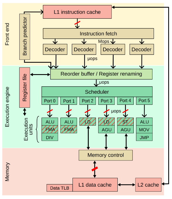
where $n_{super}^{FP}$ is the superscalarity given in instructions per cycle, $n_{FMA}$ is the FMA factor given in flops per lane, $n_{SIMD}$ is the SIMD factor given in lanes per instruction and $f$ is the clock speed given in cycles per second. Figure 1 shows the anatomy of a modern CPU core, where there are multiple cores per Core Complex (CCX), all sharing an L3 cache. This core, similar to an AMD EPYC Milan node, has 2 FMA execution units, which are general purpose FP execution units, each with 256-bit registers that can be decomposed into 4 FP64 SIMD lanes or 8 FP32 SIMD lanes.
The memory hierarchy was then discussed, as the main limiting factor to performance rather than in-core parallelism. Node topology was discussed, introducing the concepts of the socket and ccNUMA (cache coherent non-uniform memory access) nodes. This naturally led to the introduction of the Roofline model as a method of characterising scalability in a code based on the architecture it is running on. Further more it provides an indication about whether a code is operating as memory bound or compute bound. The Roofline model is a graph of performance (in FLOPs/s) against computational intensity (in FLOPs/byte), where a FLOP is a Floating-point Operation. The initial slope is determined by the memory bandwidth multiplied by the computational intensity. The “roof” is simply the peak theoretical throughput in FLOPs. The Roofline model can be a useful diagnostic tool for kernels.
In the next session, a few tools are mentioned for performance analysis, profiling and
engineering, however, the LIKWID toolkit is focused on for the remainder of the day.
The benefit of process pinning for memory affinity is outlined before looking into the
tools used for pinning. Two of such examples are the OpenMP pragma OMP_PLACES
with OMP_PROC_BIND and likwid-pin. The use of hardware counters was
also discussed to profile performance. LIKWID provides a preconfigured list of
hardware counters with likwid-perfctr -a. Then, a section on coding for ccNUMA
data locality was presented that touched on the idea of a “first touch” initialisation
of a data array by the threads as a method of getting the best data locality. OpenMP
SIMD instructions were discussed next. This pragma enforces vectorisation
in the compilation and can be combined with REDUCTION or DO.
Functions and subroutines can also be declared as SIMD safe and then called from within
a OMP SIMD region. This is done with !$OMP DECLARE SIMD. An important
consideration is that the effectiveness of SIMD decreases for each cache level that
the data size being operated on surpasses. This is of course due to the bottleneck
of memory transfer between cache levels and memory.
Finally, in a hands on session, we analysed the data traffic of a dense matrix-vector multiplication (DMVM). This session introduced the idea of blocking to fit data into cache more effectively and thereby reducing unnecessary data traffic. This can make a significant difference for throughput on a single core. Blocking can also have a significant impact on the OpenMP parallelised code as well. This scales reasonably, maintaining a modest improvement over unblocked code, until it approaches the bandwidth limit of the main memory, occurring at large numbers of threads/cores, which then becomes the bottleneck.
OpenMP Offloading with AMD
This session was run by AMD and was mostly a hands-on session, working with a cluster
of their new MI300A APU (Accelerated Processing Unit) to practice OpenMP offloading
of simple kernels. The MI300A benefits from CPU and GPU on chip with a unified shared
memory and is designed for HPC workloads. The main benefit to the APUs is the reduction
in memory management needed by the user and fewer copies of data in memory overall.
The compute units in these APUs also introduce the concept of wavefronts, which are
teams of 64 threads that execute on the same compute unit and share an L1 cache. Each
thread is deployed on a SIMD lane. To use the unified shared memory we need to set
HSA_XNACK=1 as an environment variable.
For the OpenMP programming, the following pragmas are required to utilise all of the compute units on the GPU device.
!$omp requires unified_shared_memory
!$omp target teams distribute parallel do thread_limit(1024)
The second line can be replaced with !$omp target loop. The thread limit is the
number of threads per team and should be a multiple of the wavefront size. Also
mentioned were the uses for the collapse pragma to collapse nested loops,
and setting the environment variable LIBOMPTARGET_KERNEL_TRACE=1 for debugging
and to see the utilisation of the GPU. The concept of data mapping was also
introduced to help the compiler in the case where unified shared memory was not
working as expected. You can create structured data OpenMP regions using the pragma
!$omp target data map(to:x) map(tofrom:y)
Finally, the interoperability of the HIP (heterogeneous-computing interface for portability) programming language with OpenMP was demonstrated and a comparison draw between the two approaches. The main example was a Red-Black Gauss-Seidel (RBGS) solver which was found to show performance enhancements with an optimised HIP kernel but was much simpler to program using OpenMP. The comparison of the two separate approaches and combined approach was too extensive to cover here but can be found in the slides they provided for those interested.
Keynote Talks
John McCalpin
This keynote talk given by John McCalpin was on the current architecture of modern hardware and it’s genealogy originating in the 1980s for serial, general purpose computing. This is in stark contrast to the highly parallel and specialised workloads of modern high performance computing. Given on the same day as the node-level optimisation workshop, this tied in neatly with Thomas Gruber’s session exploring data transfer bottlenecks in the cache system. In this presentation, McCalpin posits that a complete rethink of the architecture of current computer hardware is needed, optimising for highly parallelised workloads. McCalpin suggests that our current view of a flat memory address space should change and that user should have explicit architectural support to manipulate the memory space. McCalpin backed this idea up by explaining the concepts of hardware prefetches and coherence controllers, and provided statistics such as a single load from memory being equivalent to 100 FLOPs.
Alice-Agnes Gabriel
Dr Alice-Agnes Gabriel presented another keynote on their research on tsunamis and earthquake prediction and analysis. At the heart of this research was a finite element method (FEM) numerical method for the shallow wave equations which had a large number of degrees of freedom. Naturally, this resulted in the use of high performance computing infrastructure and the use of dimensionality reduction techniques such as reduced order modelling. The motivation for this research appeared to be to assess the underlying causes for tsunamis based on the earthquakes that caused them and for the creation of an early warning system where online reduced model simulations can run to predict the likelihood of a tsunami. The breadth of this research was amazing and the body of work was incredibly interesting.
Large Neural Network Training with Nvidia
This tutorial, run by Nvidia, was about the techniques employed when training large neural networks (NNs) on GPU devices. It began with a discussion on the Chinchilla Optimal to provide some context for efficient training of large NNs. The Chinchilla Optimal is a hypothesis posed recently in the literature about the ideal balance of model parameters (D) and training tokens (N). This optimal point maximises the effectiveness of a large language model (LLM) for a fixed compute budget in FLOPs. The overall finding of this work was that number of training tokens should be approximately 20 times the number of model parameters (or $D_{train} \approx 20N$) for an optimal LLM. A possible reason to go beyond this point would be that with additional training tokens, the cost per token in inference may be lowered. Also mentioned was an approximate formula for the number of FLOPs required to train a model, where $FLOPs = 6\cdot N\cdot D_{train}$.
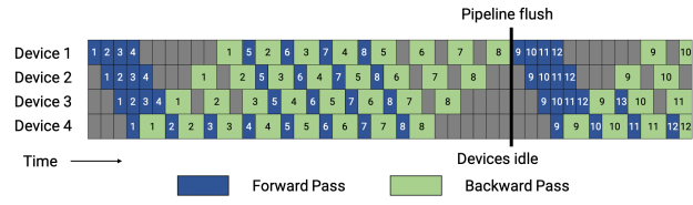
Following the Chinchilla Optimal discussion, the different forms of parallelism were introduced. The first parallelism concepts fell under Model Parallelism. These included Pipeline Parallelism (PP), Tensor Parallelism (TP) and Mixture of Experts. Additionally, Sequence Parallelism, Context Parallelism and Data Parallelism (DP) were described. Most of these techniques involved either splitting the data or the model into microbatches, with some form of gradient accumulation between the batches to keep the model consistent. Figure 2 shows an example of pipeline parallelism, with the microbatches distributed across 4 GPU devices. These techniques are all designed to reduce the amount of idle time on the GPUs and are available with Nvidia’s Megatron Bridge. The advice given was that a combination of TP, PP and DP were usually best. Most of this information is available in their documentation.
Finally, there was a discussion about the different floating point formats supported by Nvidia GPUs and their various strengths. Beyond the standard FP16 and FP8 (of which there is E3M4 and E5M2), this included the BF16, which had 8 bits for the exponent and 7 for the mantissa (as opposed to the 5 and 10 respectively in FP16). This format allows for a greater dynamic range, which can be helpful for storing gradients. Unique Nvidia floating point representations of MXFP8 and NVFP4 were also presented with a suggestion that they are better for NN training and inference, utilising more of a GPU device.
General advice about training NNs was offered during the session. For example, given how data hungry GPUs can be, tuning the data loader can often yield good improvements. Pinning memory may also help. A symptom of a data starved GPU might be bursty CPU activity. Another piece of advice was that the most memory intensive section of training NNs is the calculating the gradient of the loss function during back propagation. A potential mitigation for this could be check-pointing certain gradients and deleting most others when used. This can lead to more computation but is often worth the trade-off.